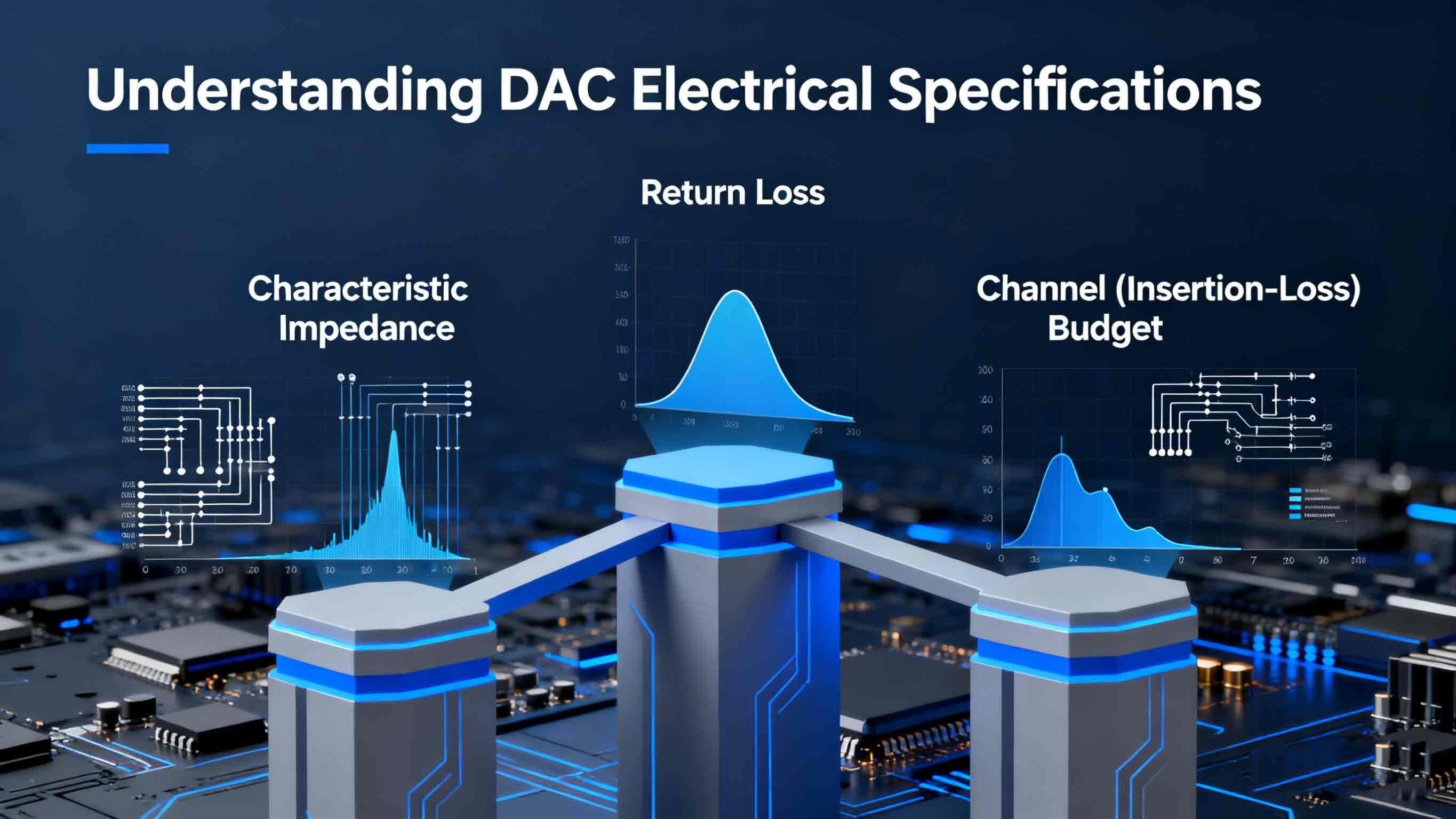
Understanding DACElectrical Specifications is essential when designing, qualifying, or buying short-reach copper links for racks and adjacent racks. This article explains the three pillars you must master — characteristic impedance, return loss, and the channel (insertion-loss) budget — and shows how they interact to determine whether a Dac Cable will behave reliably at the intended data rate.
Why these three specs matter
The electrical behavior of a Dac Cable is not an afterthought: it defines signal fidelity, equalization need, and ultimately bit-error-rate performance. Characteristic impedance mismatches create reflections; poor return loss metrics mean those reflections are large; and excessive insertion loss (the channel budget) reduces signal amplitude and forces the transceiver to apply more equalization or rely on FEC. Together, these three items are the core of any DACElectrical Specifications evaluation.
Characteristic impedance
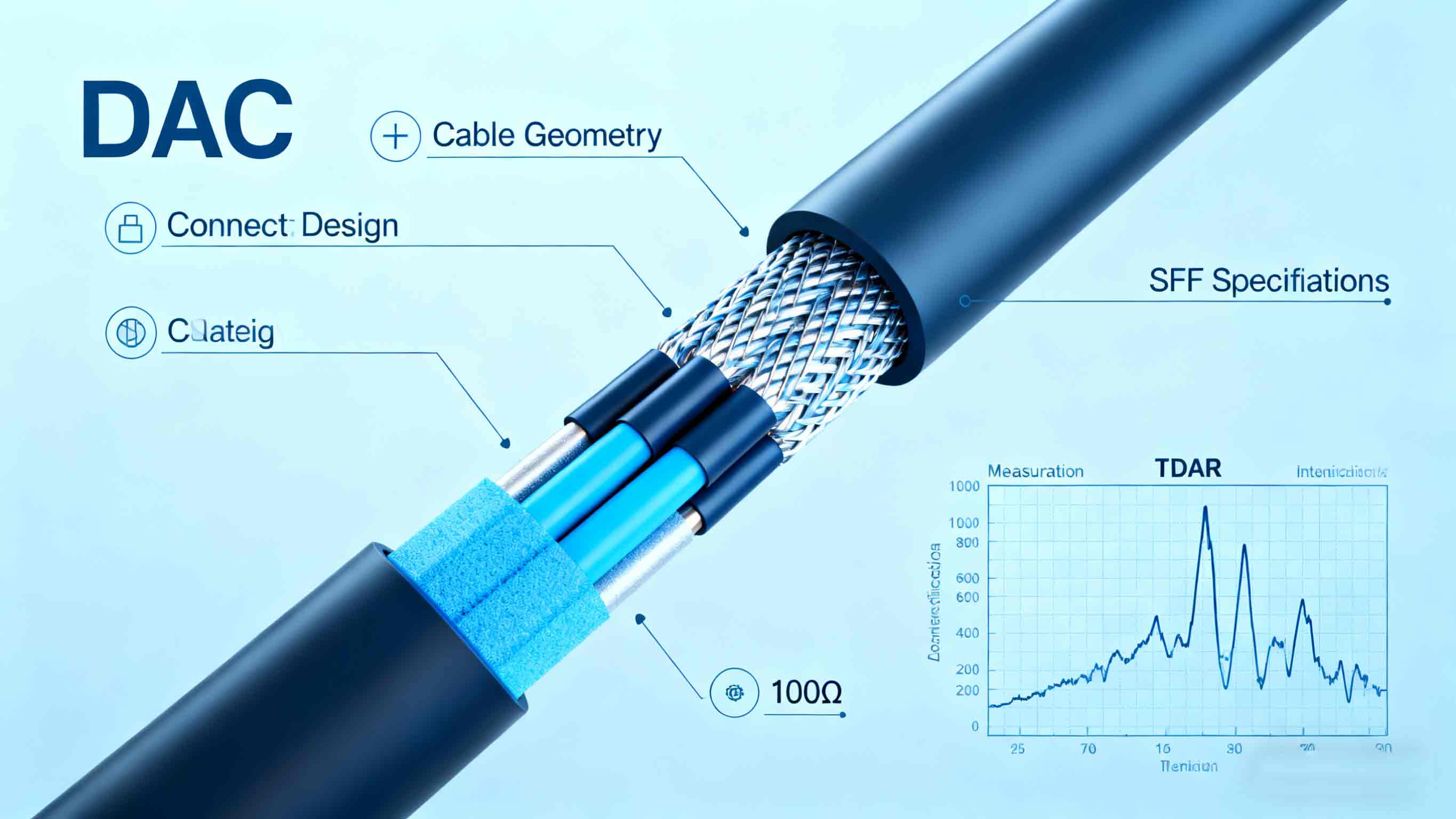
High-speed serial links use differential pairs that should target a defined characteristic differential impedance. For modern pluggable and DAC cable interfaces the industry standard target is a 100-ohm differential characteristic impedance (with tight tolerances such as ±5 Ω commonly specified). Meeting that target minimizes reflections at mating interfaces and preserves the eye. This 100 Ω target is specified in the SFF electrical guidelines used for SFP+/QSFP form factors.
Practically, impedance is controlled by cable geometry (pair spacing, conductor size, dielectric constant) and connector/PCB interface design. Manufacturers list differential impedance on data sheets; acceptance tests use a network analyzer or time-domain reflectometer (TDR) to verify that the mated assembly maintains the target impedance across the relevant frequency band.
Return loss — how reflections are quantified
Return loss (both differential and common-mode) measures how much of the launched signal is reflected back toward the transmitter due to impedance discontinuities. It’s expressed in dB; more negative numbers mean worse return loss (i.e., more energy is reflected). Return-loss specifications are frequency dependent because discontinuities and connector behavior vary with frequency. SFF-8431 and related product specifications provide frequency-based return-loss masks that vendors use to qualify DAC cable assemblies.
Two practical points:
-
Differential return loss affects the serial eye directly and increases intersymbol interference when poor.
-
Common-mode return loss matters for EMI and how the system cancels unwanted noise; inadequate common-mode return-loss performance can raise emissions and disturb adjacent circuits. Vendors often provide algebraic masks (dB vs frequency) that a cable and connector must meet.
Channel budget (insertion loss)
Channel insertion loss is the total attenuation of the transmitted signal across the entire link at the signaling frequency (or across its spectral envelope). The “channel budget” is an allocation of allowable insertion loss broken down among cable conductor loss, connector loss, host connector and PCB losses, and margin. For high-rate systems (for example QSFP28 100G electrical channels) vendors commonly design channel budgets in the tens of dB at the Nyquist or fundamental frequency used for equalization. For example, a 100G QSFP28 passive channel example allocates roughly 35 dB channel insertion loss at ~12.89 GHz for certain passive twinax assemblies.
Standards workgroups have recommended practical objectives too: analyses for 100G electrical cables cited a 30 dB loss objective for typical short (≈2 m) direct-attach copper assemblies, a useful ballpark when comparing vendor data. That target is useful when choosing a DAC cable for 25/50/56/100 Gbps lanes where loss rises rapidly with frequency.
How to read a channel budget
A simplified channel budget shows how a system arrives at a total allowable loss:
-
Transceiver equalizer budget (what the receiver can compensate): implicit in component selection.
-
Connector insertion loss (per mated connector): typically 0.5–1.2 dB depending on design; some vendor test fixtures show connector loss ≈1.07 dB.
-
Cable conductor loss (per meter): grows with frequency; a 1–2 m passive twinax at 25–50 GHz effective spectral content can contribute multiple dB.
-
Host PCB and socket allocations: often a few dB.
-
Margin: reserve (commonly 3–6 dB) for aging, temperature, and assembly variation.
Using a vendor example: a QSFP28 passive twinax datasheet showed a 35 dB channel insertion-loss budget at 12.8906 GHz with connector insertion loss around 1.07 dB and a host connector allocation of ~0.62 dB; those numbers let an engineer decide if a particular cable length and gauge will fit the budget. If the sum of measured losses exceeds the budget, the link will need active equalization or a shorter cable.
Measurement and acceptance: what to test
To verify DACElectrical Specifications in production or acceptance testing, perform:
-
Impedance profile (TDR) across the mated assembly to confirm 100 Ω ± tolerance.
-
Return loss (S11/S22) swept across the frequency band and compared to the relevant SFF mask.
-
Insertion loss (S21) to place the cable in the channel budget — ideally measured at the signaling harmonic frequencies used by the transceiver. Measurement systems from test vendors are built to automate IL/RL reporting.
Reports should list the differential impedance, differential/common-mode return loss curves, and insertion loss curve together with pass/fail against the chosen budget.
Key tradeoffs and design choices
-
Thicker conductors (lower AWG) reduce insertion loss but increase size and cost; they also affect impedance and coupling.
-
Shorter length is the easiest way to meet aggressive channel budgets.
-
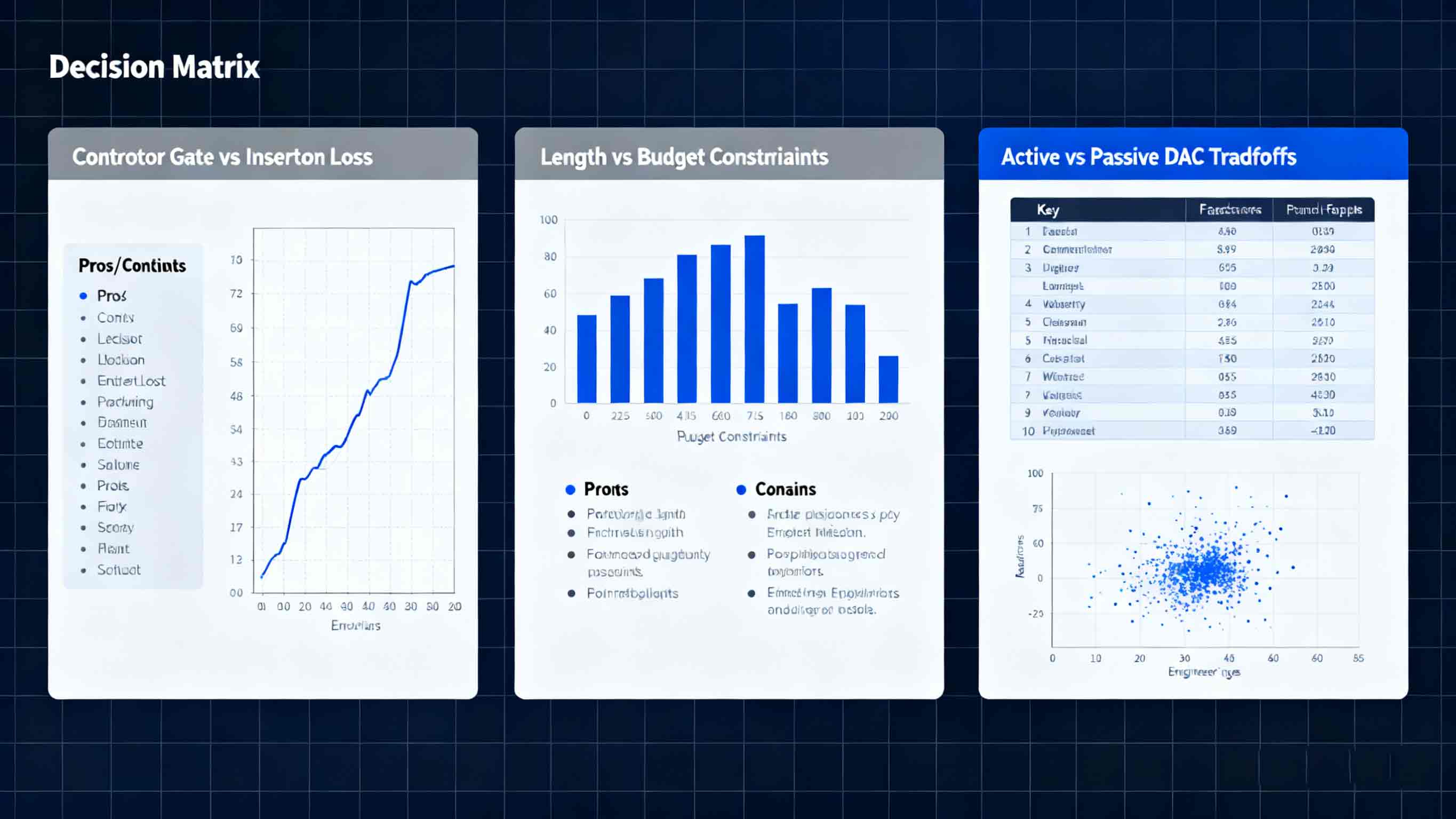
Active vs passive DAC: active assemblies can extend reach by embedding equalization, but they are more costly and can affect interoperability. Choose based on whether your design needs conservative pre-FEC margin or relies on FEC to mask marginal pre-FEC channels. Industry guidance and system architects often prefer pre-FEC margin when possible.
Conclusion
Good DAC Electrical Specifications discipline starts by insisting on a 100 Ω differential target, verifying return-loss masks across the frequency band, and computing a realistic channel insertion-loss budget that includes connectors, host allocations, and margin. When you read a datasheet or compare suppliers, map their impedance, return loss curves, and insertion-loss numbers against your channel budget and required data rate before accepting a DAC cable for production. That disciplined, numbers-first approach prevents surprises in the lab and in-service failures.